Theoretical background
Magnetic field evolution on the solar surface
The surface flux transport (SFT) model, which solves the radial component of the magnetic field on the solar/stellar surface, has demonstrated remarkable effectiveness in simulating the dynamics of the large-scale magnetic field on the solar photosphere. The governing equation can be written as,
where \(\eta\) is the magnetic diffusivity, \(\Omega (s)\) is the angular velocity in east-west direction on a uniform latitude grid, \(u_\theta\) is the flow profile along north-south direction on a latitude grid and \(\phi\) is the longitude. The velocity profiles involved in transporting the magnetic flux on the photosphere is a function of latitude only. The flux from newly emerging sun/star spots are coupled to the model via an ad-hoc source term \(S\).
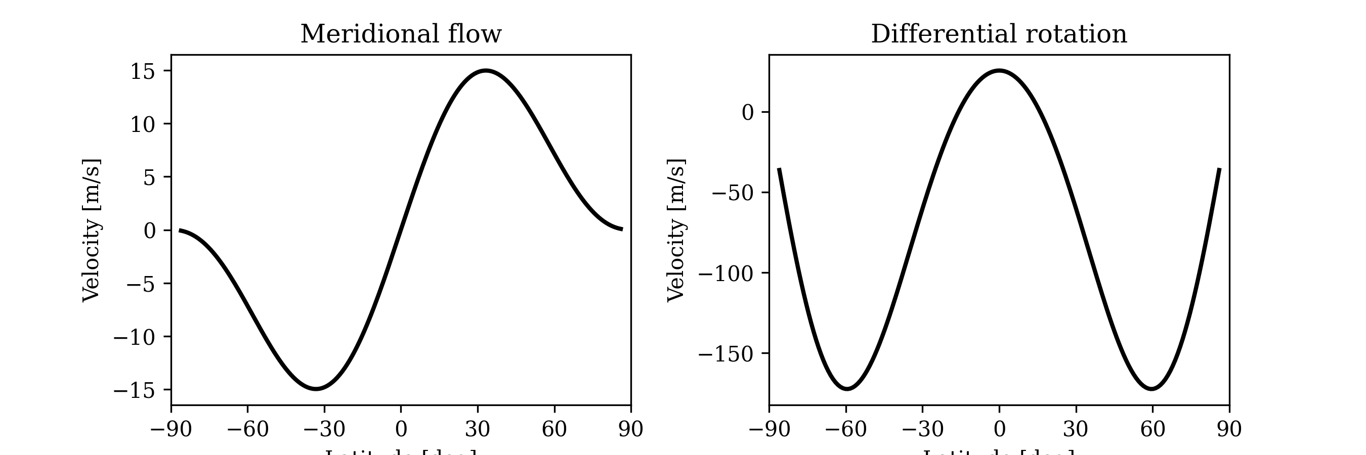
Example meridional flow profile.
Bipolar Magnetic Region (BMR) Flux Injection — Theoretical Explanation
Here is how we model the bipolar magnetic region (BMR) source term in our SFT simulation.
It describes how a pair of magnetic polarities (leading and following) is injected on the solar/stellar surface, following Joy’s law tilt and Hale’s polarity law.
The resulting field is a normalized radial magnetic field distribution representing the emergence of one BMR with a specified total flux and geometric configuration.
1. Mesh and Area Elements
The surface of the Sun is represented using a spherical grid:
The surface element on a sphere of radius ( R_\odot ) is:
This is used to compute total flux over the spherical surface.
2. Convert Center Location
The central location of the bipole in latitude \(\lambda\) and longitude \(\phi\) is converted to colatitude:
The corresponding unit vector on the sphere is:
3. Local Tangent Basis
At the emergence center, a local tangent plane is defined using orthonormal vectors:
\(\mathbf{e}_\phi\) → eastward direction
\(\mathbf{e}_\lambda\) → northward direction
4. Tilt and Separation
The tilt angle \(\alpha\) defines the orientation of the bipole line relative to the local east-west direction:
The leading and following polarity centers are positioned symmetrically along the separation vector:
where \(\Delta\) is the angular separation (in radians).
5. Convert to Spherical Coordinates
The 3D vectors are converted back to spherical coordinates:
6. Polarity Signs (Hale’s Law)
The polarity signs are determined according to hemisphere:
Optionally, Hale’s law can be disabled and the leading polarity is set positive.
7. Gaussian Field Distribution
Each polarity is modeled as a 2D Gaussian on the sphere:
where:
\(\sigma\) → angular width of the polarity
\(s_i = \pm 1\) → polarity sign
The combined unscaled radial field is:
8. Flux Normalization
Compute the total unsigned flux:
Scale the field to match the specified total flux ( \Phi ):
The normalized radial field is then:
ensuring:
9. Final Equation
The normalized radial magnetic field of the bipole is:
This is the mathematical representation of the BMR source term used in surface flux transport simulations.
10. Summary
Represents idealized BMR emergence on the solar surface.
Incorporates Joy’s law tilt and Hale’s law polarity orientation.
Normalized to ensure the total unsigned flux equals the specified value.
Provides a smooth Gaussian representation suitable for numerical simulations.
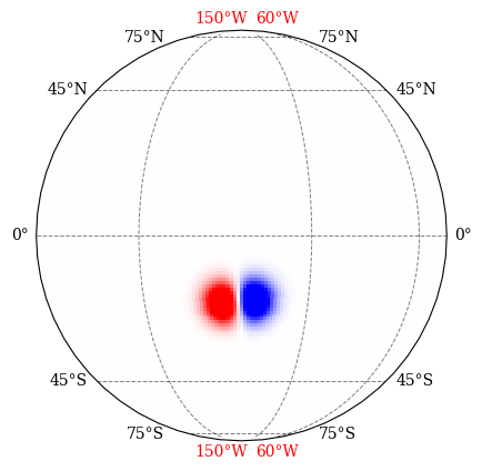
Example modeled BMR.