Theoretical background

Magnetic field evolution on the solar surface

The surface flux transport (SFT) model, which solves the radial component of the magnetic field on the solar surface, has demonstrated remarkable effectiveness in simulating the dynamics of the large-scale magnetic field on the photosphere. The governing equation can be written as,

\[\frac{\partial B}{\partial t} = \frac{D}{R_\odot^2}\left[\frac{\partial}{\partial s}\left((1-s^2)\frac{\partial B}{\partial s}\right) + \frac{1}{1-s^2}\frac{\partial^2B}{\partial\phi^2}\right] - \frac{\partial}{\partial s}\left[\frac{v_s(s)}{R_\odot}\sqrt{1-s^2} B\right] - \Omega(s)\frac{\partial B}{\partial\phi}\]

where \(s\) = sin\(\theta\), D is the magnetic diffusivity, \(\Omega (s)\) is the angular velocity in east-west direction on a sine-latitude grid, \(v_s (s)\) is the flow profile along north-south direction on a sine-latitude grid and \(\phi\) is the longitude. As the velocity profiles involved in transporting the magnetic flux on the photosphere is a function of latitude only, we can simplify this equation by taking average in the longitudinal direction which will improve the computational efficiency and provide us a lesser parameter space to comprehensively explore the dynamics. After averaging the \(B_r\),

\[\overline{B}(s,t)=(2\pi)^{-1}\int_0^{2\pi}B(s,\phi,t)\,\mathrm{d}\phi.\]

Using this reduced form of \(B_r\), we can re-write the equation as,

\[\frac{\partial\overline{B}}{\partial t} = \frac{\partial}{\partial s}\left[\frac{D}{R_\odot^2}(1-s^2)\frac{\partial\overline{B}}{\partial s} - \frac{v_s(s)}{R_\odot}\sqrt{1-s^2}\overline{B}\right],\]

where the north-south velocity is, \(v_s(s) = D_us(1-s^2)^{p/2}.\) In this form the velocity, \(s\) = sin\(\theta\) and \(D_u\) controls the amplitude of the function.

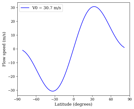
Example meridional flow profile.

BMR modeling algorithm

We follow the Bipolar Magnetic Region (BMR) modeling algorithm described in Yeates (2020) to incorporate BMRs in SFT model using observed SHARP parameters. The location of the is modelled with the positive and negative polarity positions \((s_+, \phi_+)\) and \((s_-,\phi_-)\) on the computational grid. Here \(s\) denotes sine-latitude and \(\phi\) denotes (Carrington) longitude. Different properties of the source functions are modeles as following,

1. Centroid of the BMR,

\[ s_0 = \frac12(s_+ + s_-),\qquad \phi_0 = \frac12(\phi_+ + \phi_-) \label{eqn:center}\]

2. Polarity separation, which is the heliographic angle,

\[ \rho = \arccos\left[s_+s_- + \sqrt{1-s_+^2}\sqrt{1 - s_-^2}\cos(\phi_+-\phi_-) \right] \label{eqn:separation}\]

3. The tilt angle with respect to the equator, given by,

\[ \gamma = \arctan\left[\frac{\arcsin(s_+) - \arcsin(s_-)}{\sqrt{1-s_0^2}(\phi_- - \phi_+)}\right] \label{eqn:tilt}\]

Together with the unsigned flux, \(|\Phi|\), these parameters define the BMR as following. For an untilted BMR centered at \(s=\phi=0\), this functional form is defined as

\[ B(s,\phi) = F(s,\phi) = -B_0\frac{\phi}{\rho}\exp\left[-\frac{\phi^2 + 2\arcsin^2(s)}{(a\rho)^2}\right], \label{eqn:bmr}\]

where the amplitude \(B_0\) is scaled to match the corrected flux of the observed region on the computational grid. To account for the location \((s_0,\phi_0)\) and tilt \(\gamma\) of a general region, we set \(B(s,\phi) = F(s',\phi')\), where \((s',\phi')\) are spherical coordinates in a frame where the region is centered at \(s'=\phi'=0\) and untilted.

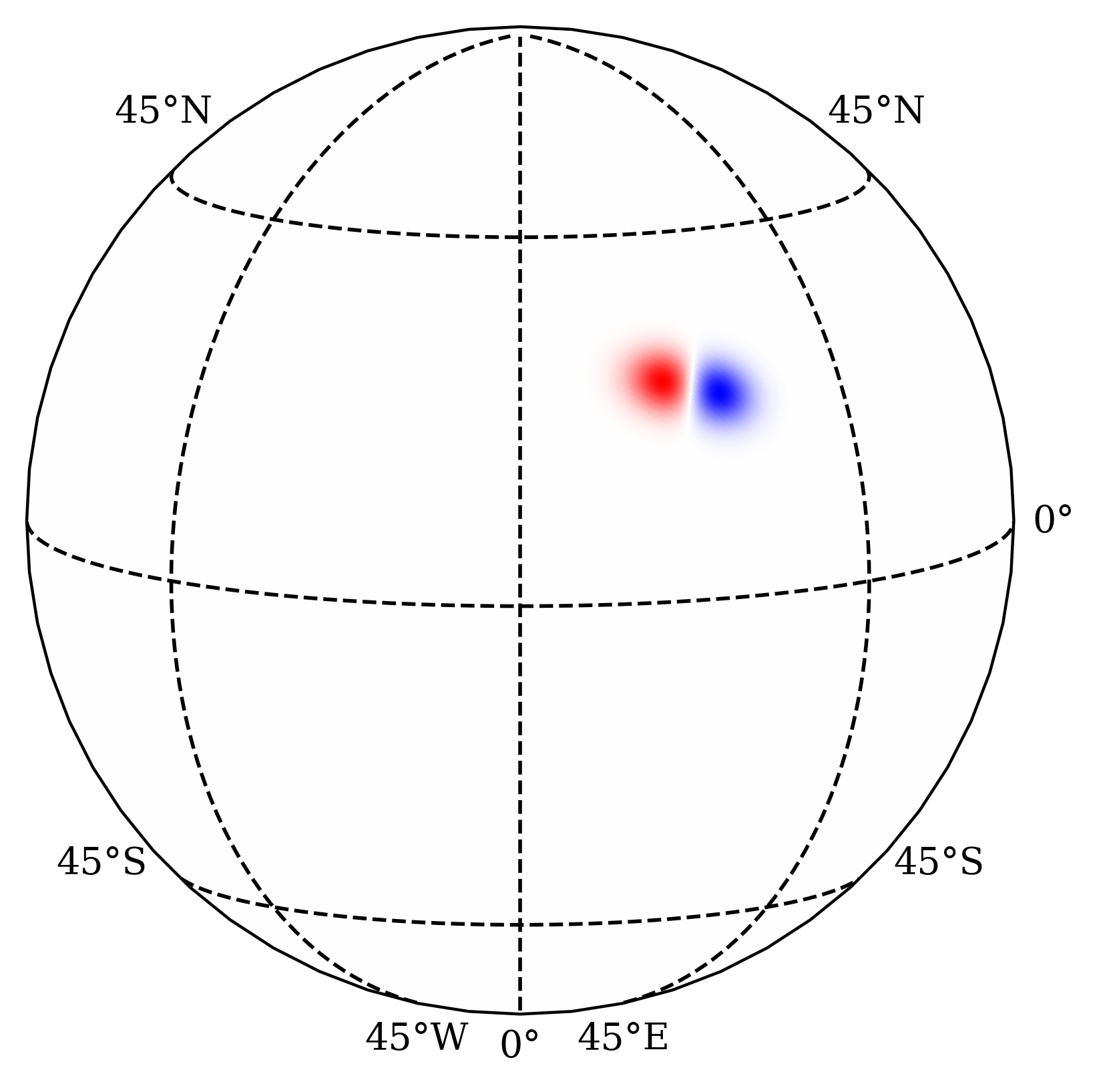
Example modeled BMR.