Sample plotting routine for SFT 1D

Here is an example of the plotting the outputs from Surface Flux Transport model 1D.

import numpy as np
import matplotlib.pyplot as plt
from mpl_toolkits.axes_grid1 import make_axes_locatable
from matplotlib import rc
import matplotlib.style
#plt.ion()
## Plotting canvas properties.
params = {'legend.fontsize': 12,
          'axes.labelsize': 12,
          'axes.titlesize': 12,
          'xtick.labelsize' :10,
          'ytick.labelsize': 10,
          'grid.color': 'k',
          'grid.linestyle': ':',
          'grid.linewidth': 0.5,
          'mathtext.fontset' : 'stix',
          'mathtext.rm'      : 'DejaVu serif',
          'font.family'      : 'DejaVu serif',
          'font.serif'       : "Times New Roman", # or "Times"
         }
matplotlib.rcParams.update(params)

from scipy.io import netcdf_file
import os
import pickle
import glob
import datetime
from datetime import datetime as dt1
from datetime import timedelta
import f90nml

Set the time range for the plot.

t_sft = np.arange(dt1(2010,6,17), dt1(2024,6,14), timedelta(days=1)).astype(dt1)

Function to convert time string to fractional year.

def frac_year(time_string):
    SECONDS_IN_DAY = 60.0*60.0*24.0
    SECONDS_IN_YEAR = SECONDS_IN_DAY*365.25
    t1 = datetime.datetime.strptime(time_string, '%Y-%m-%d') #stime.parse_time(time_string)
    t1_diff = t1 - datetime.datetime(t1.year,1,1,0,0,0)
    frac_year = (t1_diff.days + t1_diff.seconds/(60*60*24.0))/365.25
    return t1.year + frac_year

Create a plot dir to save the results.

PLOTPATH = os.getcwd()+'/plots'
if not os.path.exists(PLOTPATH):
    os.makedirs(PLOTPATH)

Read the parameter file to retrive the values

nml = f90nml.read('initial_Parameters.nml')
eta = nml['user']['eta']

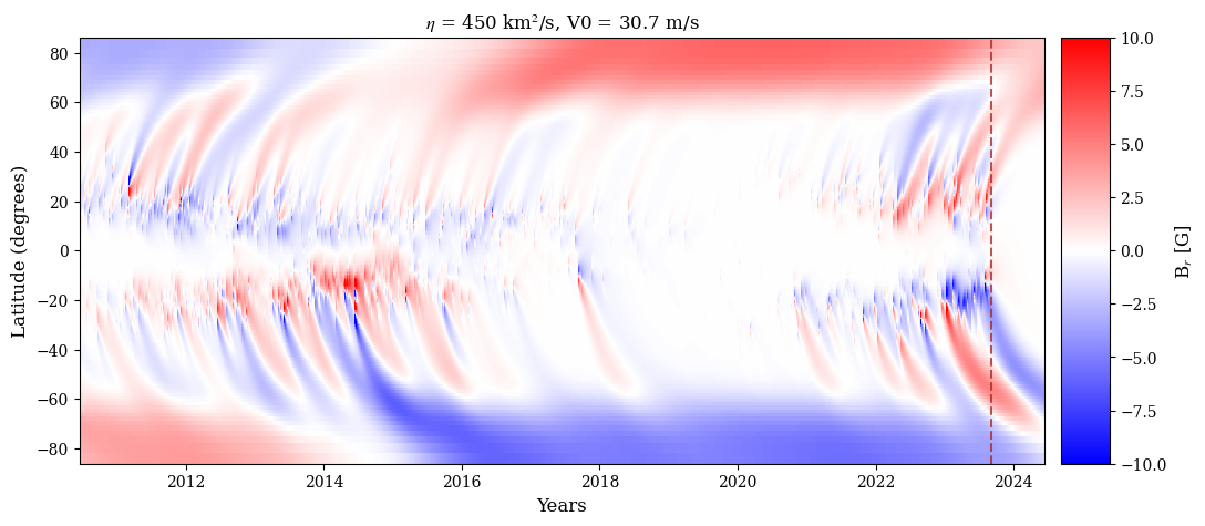
Read the butterfly diagram file from the output directory.

bfly1 = glob.glob(os.getcwd()+'/output_files/bfly_%3d_*.nc'%int(eta))[0]

fh2 = netcdf_file(bfly1)
bfly = fh2.variables['bfly'].data.copy()
sth = fh2.variables['sth'].data.copy()
time = fh2.variables['time'].data.copy()

fh2.close()

# Plot the butterfly diagram for the SFT simulation output
fig = plt.figure(figsize=[12,5])
ax1 = plt.subplot(111)

vel = glob.glob(os.getcwd()+'/output_files/MC_vel*.dat')[0]
v1 = np.loadtxt(vel)
L1 = 6.96e5
print('%2.1f'%(np.max(v1[:,1])*L1*1E3))
pm = ax1.pcolormesh(time,np.rad2deg(np.arcsin(sth)),bfly,cmap='bwr',vmax=10,vmin=-10)
ax1.set_xlim([time[0],time[-1]])
# ax1.set_xlim([-90,90])
ax1.set_xlabel('Years')
ax1.set_ylabel('Latitude (degrees)')
ax1.axvline(x = frac_year('2023-09-04'), c='brown',ls='--',alpha=0.8)
divider = make_axes_locatable(ax1)
cax = divider.append_axes('right', size='5%', pad=0.15)
fig.colorbar(pm, cax=cax, orientation='vertical',label='B$_r$ [G]')
ax1.set_title('$\eta$ = %3d km$^2$/s, V0 = %2.1f m/s'%(int(eta),np.max(v1[:,1])*L1*1E3))

# plt.savefig(PLOTPATH+'/bfly_all_bipoles_450_155.png',
#             dpi=300,transparent=False,bbox_inches='tight')
plt.show()

30.7

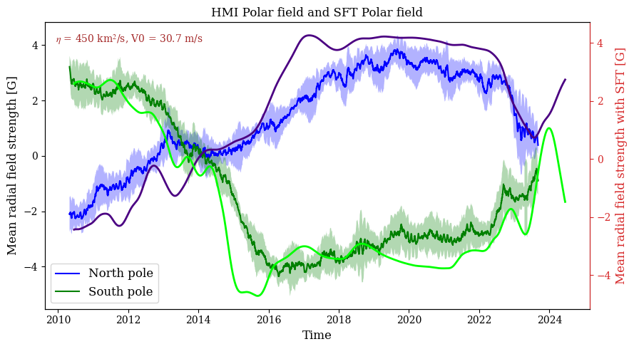
Plot and compare the HMI polar field data with SFT simulation output. The HMI observations are written to a pickle file and distributed along with the model for easy access.

picklefile = open(os.getcwd()+'/hmi_polar_field.p','rb')
n = pickle.load(picklefile)
s = pickle.load(picklefile)
mn = pickle.load(picklefile)
ms = pickle.load(picklefile)
sn = pickle.load(picklefile)
ss = pickle.load(picklefile)
t = pickle.load(picklefile)
picklefile.close()


# Plot raw data
fig, ax = plt.subplots(1, 1, figsize=(9, 5))
ax.fill_between(t, mn - sn, mn + sn, edgecolor="none", facecolor="b", alpha=0.3, interpolate=True)
ax.fill_between(t, ms - ss, ms + ss, edgecolor="none", facecolor="g", alpha=0.3, interpolate=True)
ax.plot(t, mn, "b", label="North pole")
ax.plot(t, ms, "g", label="South pole")

ax2 = ax.twinx()
ind = np.where(np.rad2deg(np.arcsin(sth)) > 60)[0][0]

ax2.plot(t_sft,np.sum(bfly[ind:,:],axis=0)/np.shape(bfly[ind:,:])[0],lw=2,c='indigo',label='Northern hemisphere')
ax2.plot(t_sft,np.sum(bfly[0:181-ind,:],axis=0)/np.shape(bfly[0:181-ind,:])[0],lw=2,c='lime',label='Southern hemisphere')


ax2.set_ylabel("Mean radial field strength with SFT [G]", color="C3")
# ax3.set_xlabel("Time", color="C1")

ax2.tick_params(axis="y", color="C3", labelcolor="C3")
ax2.spines["right"].set_color("C3")

ax.set_title('HMI Polar field and SFT Polar field', fontsize="large")

ax.set_xlabel("Time")
ax.set_ylabel("Mean radial field strength [G]")
ax.legend(loc = 3)
fig.tight_layout()

ax.text(0.02,0.93,'$\eta$ = %3d km$^2$/s, V0 = %2.1f m/s'%(int(eta),np.max(v1[:,1])*L1*1E3)
        ,color='brown',fontsize=10,transform=ax.transAxes)

# plt.savefig(PLOTPATH+'/polar_field_comparision_%3d_%3d.png'%(int(eta),np.max(v1[:,1])*L1*1E4),
#             dpi=300,transparent=False,bbox_inches='tight')
plt.show()

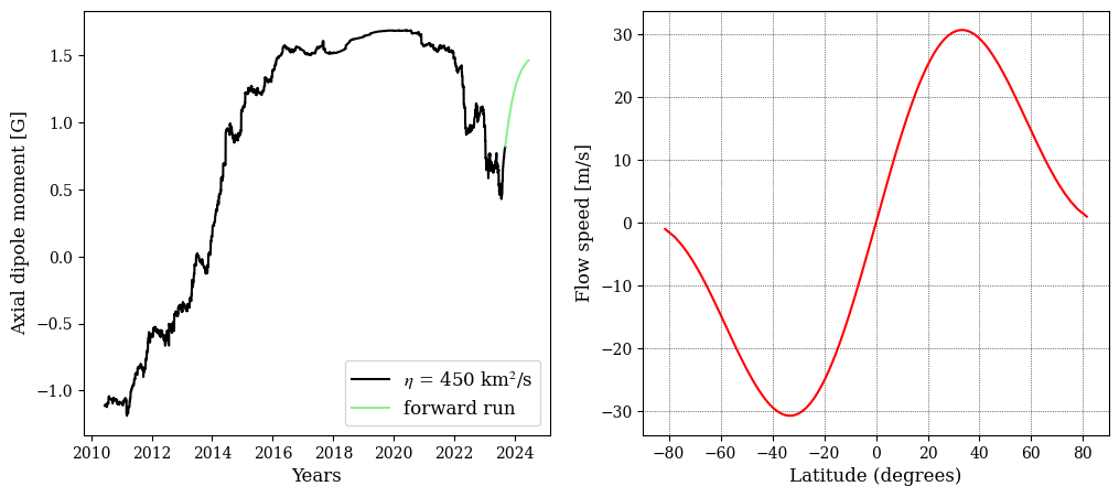
Read and plot the dipole moment and velocity profile used in the simulation.

f1 = glob.glob(os.getcwd()+'/output_files/DM_*.dat')[0]
f2 = np.loadtxt(f1)


plt.figure(figsize=[12,5])
ax1 = plt.subplot(121)
ax1.plot(time[:np.where(time >= frac_year('2023-09-04'))[0][0]],f2[:np.where(time >= frac_year('2023-09-04'))[0][0],1],label='$\eta$ = %3d km$^2$/s'%(int(eta)),c='k')

ax1.plot(time[np.where(time >= frac_year('2023-09-04'))[0][0]:-1],f2[np.where(time >= frac_year('2023-09-04'))[0][0]:,1],label='forward run',c='lightgreen')

# ax1.set_xlim([time[0],frac_year('2023-09-04')])
ax1.set_xlabel('Years')
ax1.set_ylabel('Axial dipole moment [G]')
ax1.legend()

ax2 = plt.subplot(122)
vel = glob.glob(os.getcwd()+'/output_files/MC_vel*.dat')[0]
v1 = np.loadtxt(vel)
ax2.plot(np.rad2deg(np.arcsin(v1[:,0])),v1[:,1]*L1*1E3,label='20',c='r')

ax2.set_xlim([-90,90])
ax2.set_xlabel('Latitude (degrees)')
ax2.set_ylabel('Flow speed [m/s]')
ax2.grid()
# plt.savefig(PLOTPATH+'/DM_flows_%3d_%3d.png'%(int(eta),np.max(v1[:,1])*L1*1E4),
#             dpi=300,transparent=False,bbox_inches='tight')
plt.show()